Demand-Intensity Models - Engineering Demand Parameter vs Intensity Measure

Non-linear and collapse prediction demand-intensity models

One of the greatest challenges in earthquake engineering has been accurately measuring how ductile systems respond non-linearly to dynamic forces, using only a structure's linear elastic and static properties. This fundamental concept underpins numerous seismic design codes and assessment guidelines (FEMA P58-3, SEAOC Vision 2000, Cornell and Krawinkler 2000), forming the basis for various analytical approaches. When engineers directly consider non-linear responses, methods such as non-linear static pushover analysis adjust the lateral force pattern to reveal comprehensive structural behaviour from elasticity through yielding and ultimately towards collapse.

In the 1960s, researchers developed inelastic spectra that related key parameters: the ratio to elastic spectral demand (R), ductility demand (μ), and period (T). These formed what are commonly known as R-μ-T relationships. These relationships established essential connections between a structure's elastic design strength and its expected non-linear performance during seismic events, providing engineers with practical tools for seismic design and assessment.

Those simplified non-linear static procedures are widely used by engineers and incorporated into various building codes worldwide (e.g., Eurocode 8) to evaluate the non-linear seismic response of structural systems. These methods allow for estimating the seismic response of a structure represented by engineering demand parameters (EDPs)—using its static pushover capacity under a given seismic intensity, known as the intensity measure (IM).

Alternatively, for a known EDP threshold (e.g., a limit state), these procedures can determine the seismic intensity required to exceed that threshold. This approach relies on empirical relationships between EDPs and IMs, often referred to as R−μ−T relationships. These relationships capture the complex interaction between seismic intensity, ductility demand, and the structure's vibration period, depending on the system's hysteretic behaviour and the selected IM. The API available in the Djura platform simplifies the computation of EDP-IM models for various structural systems across a wide range of vibration periods, ductility capacities, and damping ratios. It also incorporates the next-generation IM, average spectral acceleration, which has been shown to be a more efficient predictor of non-linear responses in many structural systems. This tool should make your seismic analysis both more accurate and more efficient. Let's take a closer look at how it works.

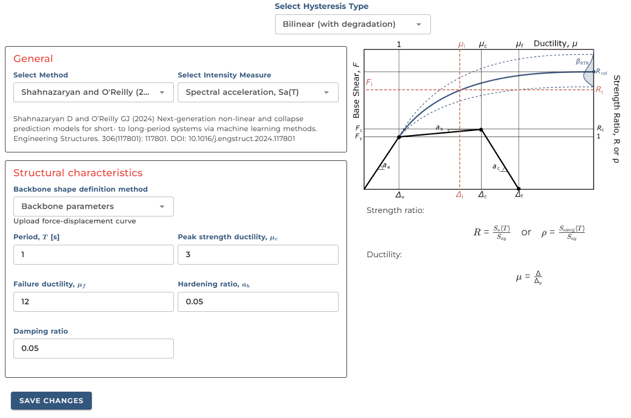
Bilinear (with degradation) models

We will first examine bilinear models. A bilinear demand-intensity model is more suitable for structural systems like reinforced concrete frames where the response exhibits distinct phases. To construct these models, we need to define a backbone curve through three distinct points:

• Yielding point (y) - where the structure begins to deform plastically
• End of plasticity (c) - marking the transition to strength degradation
• Fracturing point (f) - representing ultimate failure

These key points are shown in the figure below and are necessary to construct the backbone shape or the idealised static pushover curve, which is essential for estimating the demand-intensity response of the system. The backbone curve effectively captures how the structure will respond to increasing seismic forces, from initial elastic behaviour through yielding and ultimately to failure.

Currently Djura support multiple methods and two intensity measures (spectral acceleration and average spectral acceleration). However, the plan is to include more methods and intensity measures during the lifetime of the software.

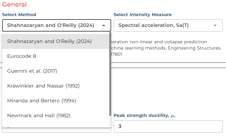
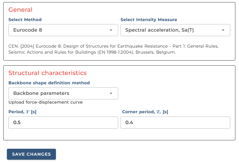
The input parameters will vary depending on the selected method. For example, in the case of Eurocode 8, we need to define the system fundamental period and spectrum corner period.

However, we will stick to the more complex approach of Shahnazaryan and O'Reilly. Here to derive the demand-intensity model, we have three choices to begin with:

1. 1. Backbone parameters
2. 2. Force-displacement backbone
3. 3. Upload force-displacement curve

We will go over each method separately.

1. Backbone parameters

One approach is to define the backbone parameters, or the force-displacement curve. For this, we must specify:

• The period of the system, (we will use 1.0)
• Peak strength ductility, (3)
• Fracturing ductility, (6)
• Damping ratio, (0.05)
• Hardening ratio, (0.05)

These parameters can be defined based on the figure and equations shown above. The force-displacement curve represents how the structure responds to lateral forces, with the hardening ratio indicating the post-yield stiffness as a proportion of the initial elastic stiffness. The ductility parameters define how much deformation the structure can undergo beyond its yield point before failure, while the damping ratio characterises the structure's ability to dissipate energy during seismic events. Together, these parameters form a comprehensive mathematical model that engineers can use to predict structural behaviour during earthquakes. Once, we are happy with the input we can click Run and derive the model.

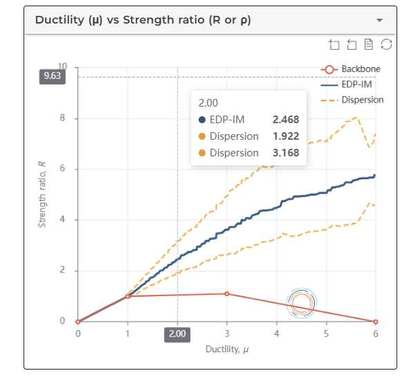
Here we have the data visualisation options (as shown in the figures below). At its fracturing point, the structure's strength ratio capacity is approximately 5.8. The 16th and 84th percentiles are also visible, providing insight into the statistical distribution of potential responses.

We can switch to the Displacement vs Force plot for greater flexibility. This alternative view allows us to assign specific displacement and acceleration values, as well as equivalent mass and first mode participation factor. This essentially gives us the flexibility to check the system's demand-intensity model according to various key structural parameters.

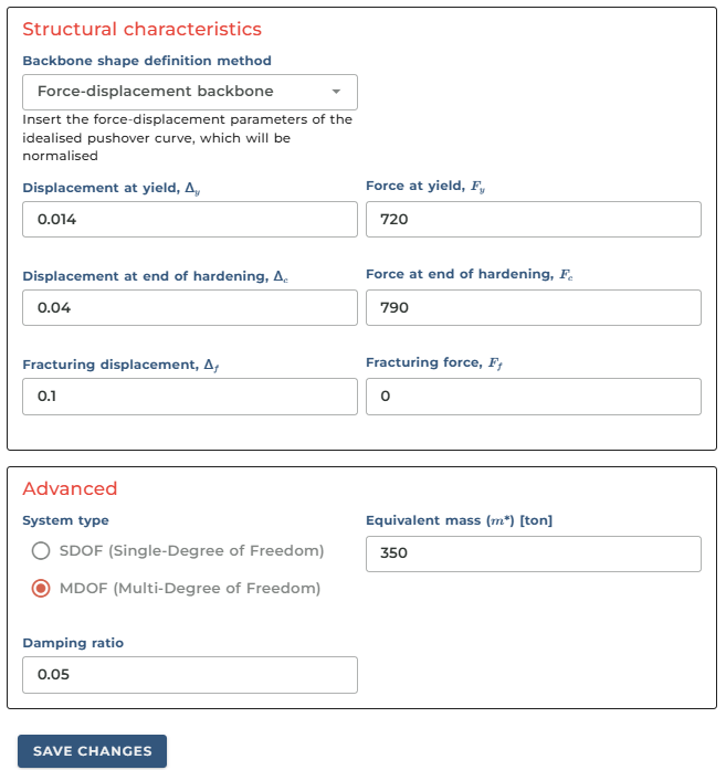
2. Force-displacement backbone

The second approach is through the use of a force-displacement backbone curve. The parameters correspond to the keys inside the figure shown before. This is essentially the idealised version of a static pushover curve. For our test, let's use the following parameters:

• Displacement at yield = 0.014
• Force at yield = 720
• Displacement at end of hardening = 0.04
• Force at end of hardening = 790
• Fracturing displacement = 0.1
• Fracturing force = 0

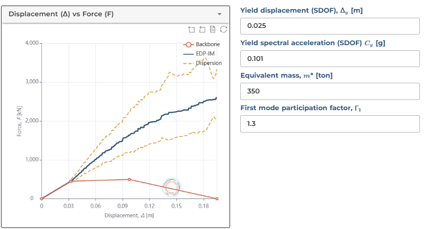
There is another type of input you may provide. We can switch to MDOF (multi-degree of freedom system), which represents a more complex structural system. In this case, we can directly provide the software with its equivalent mass and run the analysis in a similar fashion, adding an extra layer of flexibility.

Let's change to an MDOF model and assign an equivalent mass of 350 tonnes.

After saving changes and running the software, we can visualise the data in a similar way, but with additional information. For example, if we switch back to the Backbone curve through the dropdown, we'll see populated values - this is the software recalculating those values based on the provided force-displacement relationship. This approach allows for more realistic modelling of complex structures where mass distribution significantly affects seismic response behaviour.

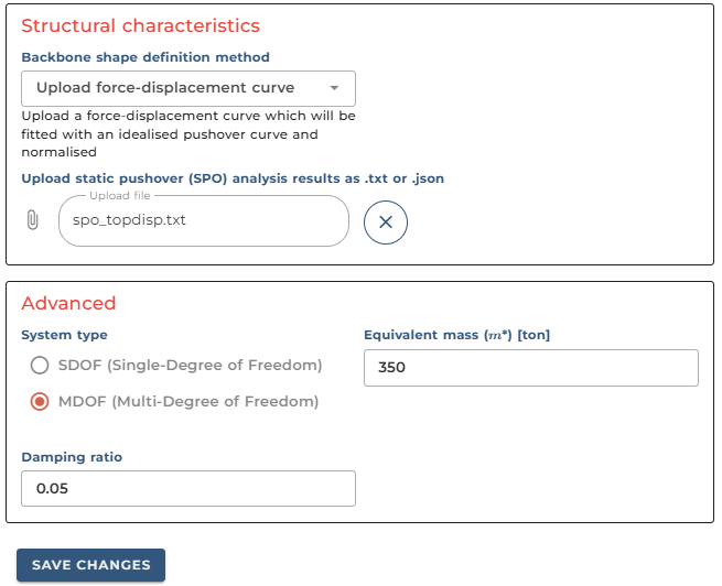
3. Upload force-displacement curve

Finally, the third approach is to directly upload a force-displacement curve. This could even be a static pushover curve obtained through any structural engineering software. The software will perform fitting on the curve and obtain the idealised pushover curve. If the fitting is not satisfactory, you may manually adjust the parameters to make the fit better.

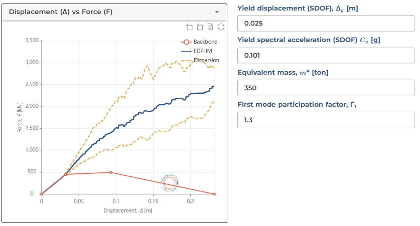
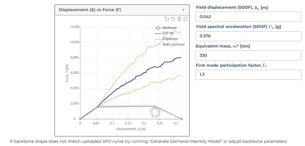
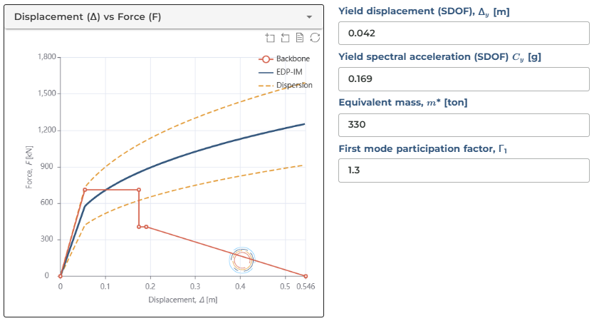
When viewing the Displacement vs Force plot, we notice our fit doesn't quite match the actual SPO curve. Hence, we need to adjust the yield displacement and equivalent mass. After setting the mass to 330 tonnes, we get a better picture.

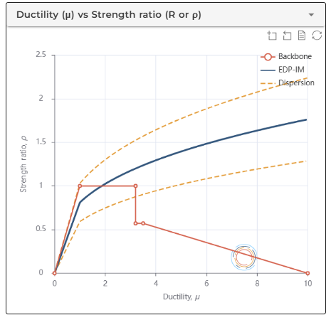
This mismatch isn't because the fit was poor, but rather because our current inputs for visualisation aren't exactly what we need them to be. Setting yield displacement to 0.042 and mass to 330, while keeping gamma at 1.3, should improve the match. When switching to the ductility vs strength ratio plot, this issue disappears. This is because the model doesn't consider the mass and the absolute values of yield displacement and acceleration. This means you can obtain a model for your input backbone shape and apply it to any system with similar backbone shapes.

The example static pushover curve input may be downloaded here.

Some Practical Features

• You may download the estimates by clicking the download button (as shown below).
• To clear the results, simply click the X button (which clears the cache).

These interactive features make it straightforward to generate, save and reset your analysis as needed during the structural assessment process.

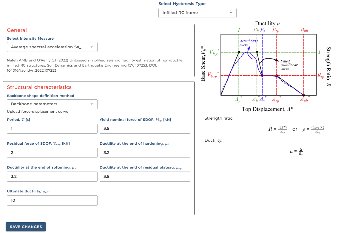
Infilled RC frame

Non-ductile masonry infilled reinforced concrete frames exhibit a distinctly different type of response compared to standard RC frames. In these structures, infill panels tend to collapse at very low drift levels in a single storey, resulting in a soft-storey response in the critical storey, while significant stiffness remains in other non-critical storeys. To capture this behaviour accurately, we need to use a specialised backbone curve that reflects this unique response pattern—which is typically how the pushover curve of such a system will appear. As with the previous models, we have three options to define the backbone parameters, but I'll demonstrate just one approach, as we've already covered the other two methods. For this model, when defined through a backbone curve, we need to specify five distinct points rather than the three required for bilinear models. This additional complexity allows us to better represent the sudden strength degradation characteristic of infill panel failure.

With the default values already filled in, we can run the analysis. For this case, we'll use average spectral acceleration as our intensity measure. The resulting capacity curves show how the structure responds through its various phases, from initial elasticity through the sudden strength drop associated with infill panel failure, followed by the remaining structural capacity of the bare frame. This approach captures the complex behaviour of these composite structural systems under seismic loading much more effectively than simpler models.

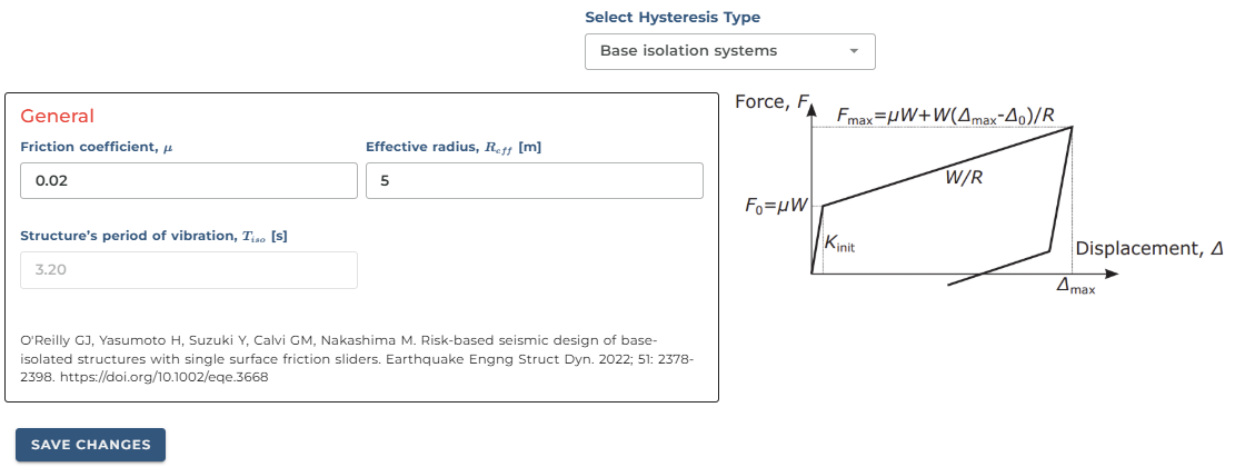
Base isolation systems

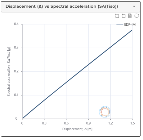
Finally, let's examine how to obtain a demand-intensity model for a friction pendulum bearing device, commonly used in base isolation systems. In this model, initial stick-slip breakaway effects are ignored, that represents the initial force required to activate the isolation system. Instead, the behaviour is governed primarily by the friction coefficient of the sliding surface (μ) and the vertical weight acting on it. Once the isolators are activated and the structure begins to slide horizontally, the structure's period of vibration becomes a function of the effective radius of curvature of the sliding surface, noted as R effective. Compared to the other two models we've examined, this one is much simpler as its response essentially depends on just two parameters. For more detailed information, you can refer to the referenced paper. If we change these parameters, the structure's period of vibration will be dynamically updated based on the new values. After saving these changes and running the app, we get the predicted demand-intensity model.

The resulting figure shows the relationship between normalised intensity (ρ) and isolator demand (δ or displacement). In logarithmic space, there's a clear linear trend between isolator displacement and the normalised intensity required to exceed it. This model has been validated through cloud analysis in a peer-reviewed publication. For additional flexibility in visualising the results, you may choose to plot displacement against spectral acceleration instead of using the normalised parameters.

Conclusion

Summary

This post explored three distinct approaches to modelling structural responses under seismic loading using simplified non-linear static procedures.

First, we examined bilinear models ideal for reinforced concrete frames, defined through backbone parameters capturing yielding, plasticity end, and fracturing points. We demonstrated multiple input methods: direct parameter definition, force-displacement curves, and uploaded pushover curves.

Next, we explored models for non-ductile masonry infilled RC frames, which require more complex backbone curves with five points to accurately represent the sudden strength loss when infill panels fail, creating soft-storey mechanisms.

Finally, we presented a simpler model for friction pendulum bearing devices used in base isolation, depending primarily on just two parameters: friction coefficient and effective radius of curvature.

Throughout, we demonstrated the flexibility of these approaches in adapting to different structural systems and varying levels of available data. The interactive visualisation tools allow engineers to readily assess seismic performance across multiple parameters, enhancing both design and assessment workflows in earthquake engineering practice.

Future Updates

We have tested this and are adding more features and flexibility so please let us know if you have specific needs. The goal is to add more models during the lifespan of the software. If you have any suggestions, get in touch with us, and we will implement them.

This tool will also be callable via API directly from Python or Matlab from your local machine so when you get comfortable, you can integrate this tool directly within your workflow with a single command.

Stay Tuned

Get in touch if we would like to use this service by visiting the website, or dropping us an email. Stay tuned for other videos and contact us for more information.

References

• Shahnazaryan D and O’Reilly GJ (2024) Next-generation non-linear and collapse prediction models for short- to long-period systems via machine learning methods. Engineering Structures. 306(117801): 117801. DOI: 10.1016/j.engstruct.2024.117801
• Nafeh AMB and O’Reilly GJ (2022) Unbiased simplified seismic fragility estimation of non-ductile infilled RC structures. Soil Dynamics and Earthquake Engineering 157: 107253. DOI: 10.1016/j.soildyn.2022.107253
• O'Reilly GJ, Yasumoto H, Suzuki Y, Calvi GM, Nakashima M. Risk-based seismic design of base-isolated structures with single surface friction sliders. Earthquake Engng Struct Dyn. 2022; 51: 2378-2398. https://doi.org/10.1002/eqe.3668
• FEMA. FEMA P58-3. Seismic Performance Assessment of Buildings Volume 3 - Performance Assessment Calculation Tool (PACT). Washington, D.C.: 2012
• S.E.A.O.C. Vision 2000: Performance-based seismic engineering of buildings 1995.
• Cornell CA, Krawinkler H. P Progress and challenges in seismic performance assessment. PEER Cent N 2000; 3(2):1–2.
• CEN. 2004 Eurocode 8: Design of Structures for Earthquake Resistance - Part 1: General Rules, Seismic Actions and Rules for Buildings (EN 1998-1:2004), Brussels, Belgium.